
What happens if you duplicate the data used in OLS linear regression?
You can encounter this problem in many forms; the one I first received was asking particularly how the t-statistic changes, but you can get it under other formulations. We look at the most common variables related to regression and how they change under the multiplied samples.
We start by taking a peek at how linear regression works, but you can skip this section and head straight to the proof if you are confident you are familiar with the concepts.
Linear Regression, Quick Recap
Linear regression aims to fit a line (or plane, or hyperplane) to the data, explaining a relationship between the dependent and independent variables. Then, we can use it to infer or forecast new values.
Formally, assume there is a linear relationship between y – the dependent variable – and x -the independent one. In the univariate case, this looks something like this, but it can be generalized to any size of vector X. We can see the regression equation, which is linear in its coefficients – beta. The remaining piece that alters this relationship is an unobserved random variable, the error term.
To proceed from here, we have to assume a series of facts about the relationships between the known and unknown variables. We do not discuss them in detail here, but I will broach how they might not hold when we double the sample size. The logical next step is to estimate the values of the parameter beta. The difference between the actual and estimated values is called the residual. We want to select the estimators in such a way that we minimize the sum of squared residuals.
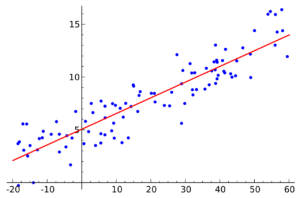
Fitting the line to the points means that, as we said before, we minimize the sum squared of residuals: red lines in this graph. Moving the line around by changing the values of beta 0 and beta 1, we can arrive at the optimal one. Intuitively, having duplicate points in the same positions should not have an impact on this line.
Solving the Problem
At this point, we know the components that can describe a regression problem, and we can start thinking better about what might charge when we duplicate the dataset.
The goal is to provide answers to the following queries:
- Does the estimated optimal function and coefficients change?
- Do the measures of quality of fit change?
- Does our confidence in our estimators change?
The first regression is modeling  .
.
The formula of the OLS estimator is the following: 
The second regression undergoes the following change in X and y, respectively: they have a copy stacked on top of the original values. The shape of the parameter beta doesn’t change. We can compare it with the previous value. Using matrix multiplication rules, compute the product of the last two terms since matrix multiplication is associative. Each element is double the corresponding one in the matrix  , producing a change in the formula for the first regression. How do the remaining components of the formula change?
Now that we know how to multiply stacked matrices, we get the result quickly: double the corresponding product from the initial formula. But this is before inverting the product! So the first element is half the one above. By combining the two, we obtain the same OLS estimator as when training over the original dataset.
As we intuited when looking at the drawing, the estimators do not change. There is no new information added! Nevertheless, are they better at estimating the values of y? Can they even be, given that we add no additional information? Is the change in sample size enough to have an impact here?
The goodness of fit measure summarises the discrepancy between the observed and predicted values. The most famous and used is the coefficient of determination, or the so-called R squared. It measures the proportion of the variation in the dependent variable that is predictable from the independent ones. From only this commentary, it intuitively follows that regression-2 does not explain more of the variance in y than regression-1.
Using the definition of R squared in a regression frame of reference (1- Unexplained variance divided by the Explained variance), we write it as:


If the predictions were perfect, the unexplained variance would be 0, and R squared would be 1. Conversely, if the model predicts only the mean of the independent variable, the coefficient of determination would be 0. Predominantly, the values are situated in the interval [0,1], with few exceptions for inappropriately chosen models.
With the context set, we can check if the intuition that R squared is invariant holds up. Since the regression equation is the same, the predictions are as well. At the same time, the mean of y stays constant. So the R Squared is constant under data duplication.
One drawback of this measure is that it is susceptible to inflation caused when adding new explanatory variables. One attempt at solving this problem is the correction proposed by Mordecai Ezekiel, which divides each sum of squares by the corresponding degrees of freedom(N-1 and N-p-1).
Since the formula uses the degrees of freedom, the value of the adjusted R square might change due to data duplication. N, the sample size is doubled, but the number of features is the same. The adjustment coefficient for the second regression increases, resulting in a larger adjusted R squared.
One thing to remember is that beta-hat merely estimates the values governing the linear relationship between y and X. This means we want to measure how confident we are in them. The most common measure is a 1-alpha confidence interval. We need the estimate, the z-score, and the standard deviation to compute it.
Now we have to return to the ignored assumptions needed to derive the estimators. One such postulation is that the distribution of the errors conditional on the regressors is normal. Hence, the variance of y given X is sigma squared times the identity matrix.
We are fortunate enough we have a closed-form solution for the estimates of beta that we plug into the variance. Using the formula for computing the variance of constant matrix multiplication, we get the result for betas. They depend only on the matrix X and the variance of the errors given X.
There are a couple of estimates for the variance of errors, both involving the sum of squares. One divides it by the number of samples (the maximum likelihood one), and the other divides it by n-p (the unbiased one). We will use the former.
Now we can compare the estimate’s variance between the two regressions. The standard deviation of the errors is the same since we double the sum, and the denominator changes from n to 2n. The product of the matrices is the same as the one we computed before, so the variance is halved. In conclusion, when doubling the data, we reduce the standard deviation by a factor of  .
.
The changes in confidence are as follows:
- the standard error decreases by a factor of
- as well as the length of the confidence interval
- consequently, the t-statistic will increase by the same ratio, decreasing the p-value accordingly
Unfortunately, the supposed added confidence is an illusion. We did not add any new information to the model when doubling the data and are violating the necessary conditions for the linear regression needed to make these computations. While there are some areas of statistics where this practice is in use, it’s good to keep in mind that we need independence of observations to interpret the results of a least squares regression.
To put all the changes in perspective, we can load one of the many sklearn datasets and test that the changes we theorized take place: the same coefficients, and  , increased adjusted , and increased confidence in the coefficient estimates.
Testing our Result
Whenever possible, it’s ideal to test your results. We’ll go with python, as it’s the most mainstream and easily understandable option.
For our set-up, we have just a few prerequisites. We’ll use the pandas library for our data needs, sklearn will just provide a working dataset while statsmodels will do the heavy lifting.
We opted for the classical diabetes dataset and selected a set of features.
import pandas as pd
import statsmodels.formula.api as smf
from sklearn import datasets
dbs = datasets.load_diabetes()
df = pd.DataFrame(data=dbs.data,
                  columns=dbs.feature_names)
df["target"] = dbs.target
formula = "target ~ sex + bmi + bp + s2 + s3 + s5"
In order the parse the model summaries, to extract the coefficients and the goodness of fit metrics, we can use two helper functions:
def get_summary_pandas(s, h=0):
    results_as_html = s.as_html()
    return pd.read_html(results_as_html, header=h, index_col=0)[0]

def get_fit(x):
    return get_summary_pandas(x, h=None)[[2, 3]].set_index(2).to_dict()[3]
Now, with everything in place, we run the two regressions, the standard one as well as the one in which we “accidentally” copy the input data.
# Normal regression
m1_coef = get_summary_pandas(model1.fit().summary().tables[1])
m1_fit = get_fit(model1.fit().summary().tables[0])
OLS Regression Results
==============================================================================
Dep. Variable: target R-squared: 0.512
Model: OLS Adj. R-squared: 0.505
Method: Least Squares F-statistic: 76.11
Date: Sat, 17 Dec 2022 Prob (F-statistic): 1.01e-64
Time: 23:40:31 Log-Likelihood: -2388.5
No. Observations: 442 AIC: 4791.
Df Residuals: 435 BIC: 4820.
Df Model: 6
Covariance Type: nonrobust
==============================================================================
coef std err t P>|t| [0.025 0.975]
------------------------------------------------------------------------------
Intercept 152.1335 2.579 58.993 0.000 147.065 157.202
sex -227.0703 60.522 -3.752 0.000 -346.021 -108.119
bmi 537.6809 65.620 8.194 0.000 408.709 666.653
bp 327.9718 62.937 5.211 0.000 204.273 451.671
s2 -102.8219 58.063 -1.771 0.077 -216.941 11.297
s3 -291.0985 65.495 -4.445 0.000 -419.824 -162.373
s5 497.9484 66.871 7.446 0.000 366.518 629.379
==============================================================================
Omnibus: 1.439 Durbin-Watson: 2.027
Prob(Omnibus): 0.487 Jarque-Bera (JB): 1.394
Skew: 0.048 Prob(JB): 0.498
Kurtosis: 2.742 Cond. No. 33.0
==============================================================================
# Doubled regression
m2_coef = get_summary_pandas(model2.fit().summary().tables[1])
m2_fit = get_fit(model2.fit().summary().tables[0])
OLS Regression Results
==============================================================================
Dep. Variable: target R-squared: 0.512
Model: OLS Adj. R-squared: 0.509
Method: Least Squares F-statistic: 153.4
Date: Sat, 17 Dec 2022 Prob (F-statistic): 5.25e-133
Time: 23:40:31 Log-Likelihood: -4777.1
No. Observations: 884 AIC: 9568.
Df Residuals: 877 BIC: 9602.
Df Model: 6
Covariance Type: nonrobust
==============================================================================
coef std err t P>|t| [0.025 0.975]
------------------------------------------------------------------------------
Intercept 152.1335 1.816 83.764 0.000 148.569 155.698
sex -227.0703 42.624 -5.327 0.000 -310.727 -143.413
bmi 537.6809 46.215 11.634 0.000 446.976 628.386
bp 327.9718 44.325 7.399 0.000 240.975 414.968
s2 -102.8219 40.893 -2.514 0.012 -183.081 -22.563
s3 -291.0985 46.127 -6.311 0.000 -381.630 -200.567
s5 497.9484 47.096 10.573 0.000 405.515 590.382
==============================================================================
Omnibus: 3.216 Durbin-Watson: 2.029
Prob(Omnibus): 0.200 Jarque-Bera (JB): 2.789
Skew: 0.048 Prob(JB): 0.248
Kurtosis: 2.742 Cond. No. 33.0
==============================================================================
The results are in line with our expectations!
Greetings.
Want to get a powerful and fast increase in link mass? Our solution is a Xrumer blast that provides predictable growth to DR 30+ in just 7 days.
Why is this beneficial for you?
— Instant Start: You’ll see the first results within an hour.
— Predictable Growth: 1-2 processing cycles guarantee reaching DR 28-30.
— Quality Links: We use only verified and quality donors.
— Proven Cases: In our cases – 8,000+ links and 1,664+ referring domains in 48 hours.
These are not just promises, it’s a working tool. Need proof? Check out our cases by searching “Drop Dead Studio Xrumer linkbuilding” and see real testimonials and Ahrefs screenshots.
Ready to start? Place an order and get a powerful boost for your site.
The Drop Dead Studio Team